The ISCAT Proposal and ISFF Request are available to describe the scientific goals and experiment design. We went into even greater detail planning the sensor placement for ISCAT.
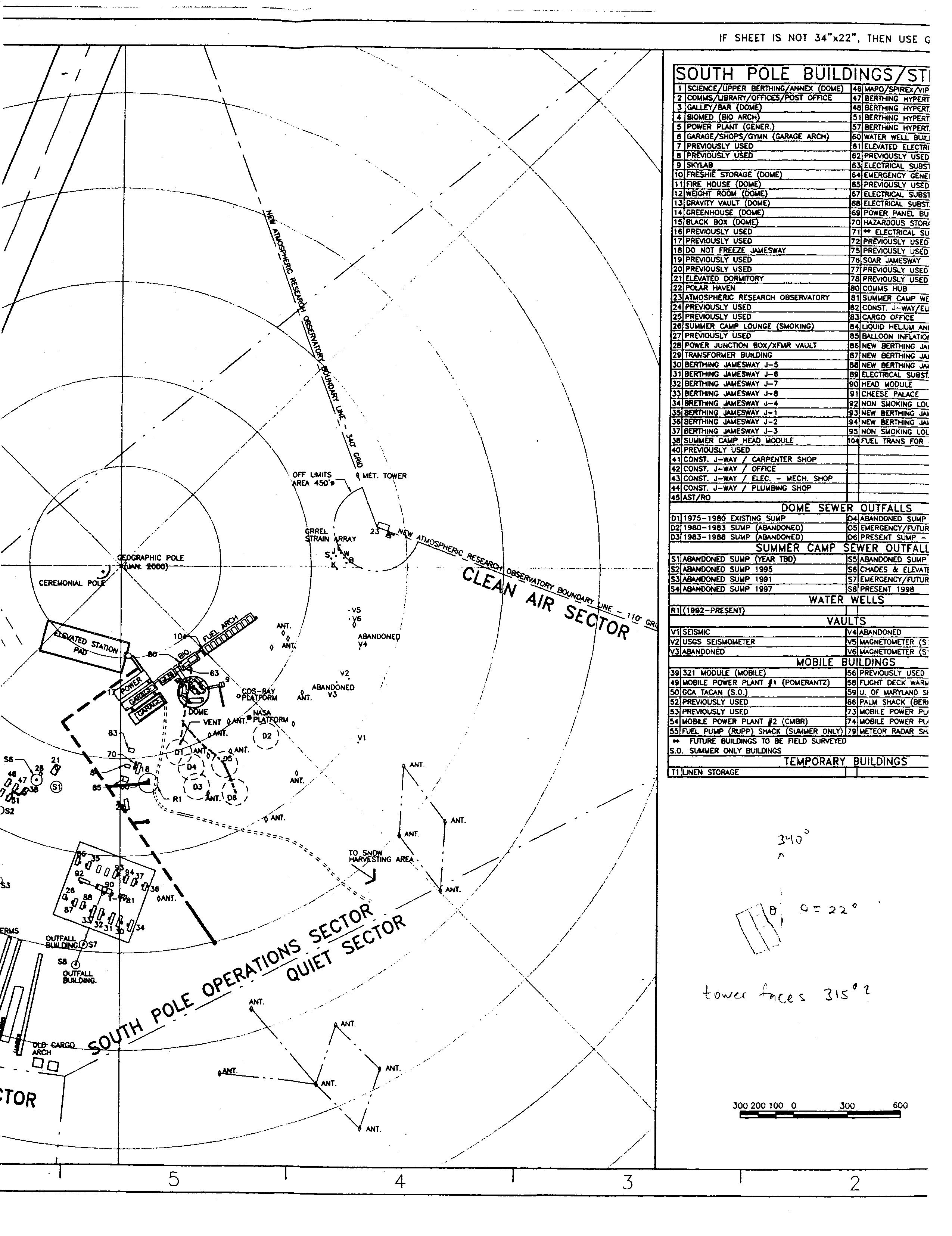
Also, data were taken near Building 23 and in the T/RH intercomparison array in addition to the normal operations array. To avoid confusion, we have decided in post-processing to split these different operations periods. Variables with a ".blg" suffix were measured near the building and with a ".ic" suffix were measured in the intercomparison array. All other data were taken in a normal mode.
Finally, one data sample at 06:40:00 on 27 Nov from the 3.1m sonic anemometer was bad, so statistics were manually recomputed for the 5-minute period contining this sample using the routine: /net/aster/isff/src/sfun/ISCAT00/fixnov27.q.
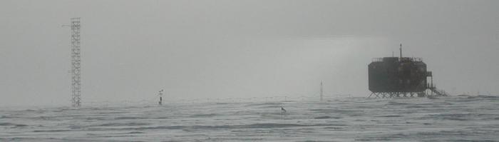
We start with a comparison of wind speed and wind direction (using our lower sonic as a reference). To obtain a bit more information, I have added the CMDL prop-vane data. (From photographs, it appears that their prop-vane was mounted at ~9.2m.) The speed from the 7.0m sonic is usually larger than those from 3.1m, as expected. The only exceptions are a few periods when the speeds are mostly less than 2.5 m/s. The CMDL prop also generally agrees with the sonic data, though the speeds are lower than expected by ~0.5 m/s. (The wind speed at 9.2m should be larger than at 7.0m.) I also note that the average speed from a prop is the average of the scalar speed magnitude, whereas the average from a sonic is the magnitude of the wind vector. Thus, the prop speed should have been even higher than the sonic speed. There is a hint in the data that the differences are largest in low winds.
To obtain agreement in wind direction, I have had to assume that the sonic anemometers were pointed in the direction of 38 degrees (rather than 70 degrees as noted in the logbook). (By scaling off a photograph and map, I obtain values from 37-40 degrees -- no, I didn't cheat!)
We can also examine our spike detector, which flags the number of data samples which are questionable. (See our Despiker documentation.) I have presented these flags as a histogram (black for 3.1m data and red for 7.0m). Only 8 5-minute periods had more than 1% of the samples flagged from the 3.1m sonic. The 7.0m sonic was significantly worse, but still only had 3 5-minute periods with more than 3% flagged as questionable. I note that our despiking algorithm can be fooled when the skewness of the data is large, which could be the case in the stable conditions during ISCAT.
Thus, at least for mean quantities, the sonic anemometer data appear to be reasonable.
We can now produce the tilt plots for the 3.1m and 7.0m sonics. Note that these plots are in actual wind direction coordinates (rather than our normal sonic coordinates). The resulting lean angles are 1.4 and 1.3 degrees, respectively, which is acceptable. The lean azimuths in this plot were computed using a (wrong) boom angle of 70 degrees, which is 160 degrees clockwise of the instrument "boom angle" of 270 degrees. Since lean azimuth is defined counterclockwise from the sonic u-vector, we must add 160 to what was computed. Thus, the lean azimuths for 3.1m are 79 deg -> 239 deg and for 7.0m are 118 deg -> 278 deg. After applying these corrections, the tilts are nearly zero for 3.1m and 7.0m.
Since a good gradient measurement was needed, the sensors were operated in an intercomparison mode at the beginning and end of the project. During the beginning IC, some sensors were exchanged (also with the spare) to obtain the best comparison. The residuals from the default calibrations were at most 0.06 C and 6% RH. However, these residuals were quite consistent during the ICs, so manual correction to 0.01 C and 1% RH probably is possible. The post-experiment ICs were done 4-channels at a time, with sensors 704 and 007 in both sets. From these two, I arbitrarily chose to reference all sensors to sensor 704 for processing the IC data.
The time periods of these ICs were:
| Pre IC#1 | 24 Nov 12:00 - 24 Nov 15:15 (NZDT) |
|---|---|
| Pre IC#2 | 24 Nov 17:00 - 25 Nov 12:40 (NZDT) |
| Post IC#1 | 27 Dec 17:00 - 28 Dec 09:00 (NZDT) |
| Post IC#2 | 28 Dec 09:45 - 28 Dec 17:45 (NZDT) |
The temperature differences (in C) from sensor 704 (the 2.1m sensor) values are:
| Sensor ID | Height Deployed | Pre IC #1 | Pre IC #2 | Post IC #1 | Post IC #2 | Used |
|---|---|---|---|---|---|---|
| 007 | 4.7m | +0.02 | +0.04 | 0.00 | +0.02 | +0.02 |
| 101 | 0.5m | +0.02 | +0.03 | +0.02 | +0.02 | |
| 104 | 0.9m | +0.03 | +0.04 | +0.03 | +0.03 | |
| 502 | 21.8m | +0.06 | +0.06 | +0.02 | +0.02 | |
| 703 | 10.1m | +0.03 | +0.03 | +0.00 | +0.00 |
and the humidity differences (in %RH) are:
| Sensor ID | Height Deployed | Pre IC #1 | Pre IC #2 | Post IC #1 | Post IC #2 | Used |
|---|---|---|---|---|---|---|
| 007 | 4.7m | +1 | +1 | +2 | +1 | +1 |
| 101 | 0.5m | -3 | -3 | -3 | -3 | |
| 104 | 0.9m | +2 | +2 | +2 | +2 | |
| 502 | 21.8m | -4 | -4 | -4 | -4 | |
| 703 | 10.1m | +6 | +6 | +6 | +6 |
We plan to remove the biases shown in the last column from the statistics (using Splus) [applied fixTRH.q, 6 Jun 01] and also from the time series processed using Java [not yet done].
Please note that the performance of our RH sensors in very cold conditions has been questioned. In particular, our sensors tended to indicate subsaturation conditions during SHEBA when conditions were thought to be saturated. A report of laboratory testing of this problem (without a satisfactory conclusion) was written for SHEBA.
The data from this sensor appear to be normal, with an average value of ~690mb. There are several data glitches early in the program (see plot), notably on Nov 22, 25, and 29, associated with data system moves and crashes (see Chronology above).
Obviously bad values will be set to NA in the final statistics data set [ran fixP.q, 7 June 01], but glitches during the above periods will still be seen in the time series. Values outside the range 675-700mb should be considered data system glitches.
| 19 | 20 | 21 | 22 | 23 | 24 | 25 |
| 26 | 27 | 28 | 29 | 30 |
| 1 | 2 | |||||
| 3 | 4 | 5 | 6 | 7 | 8 | 9 |
| 10 | 11 | 12 | 13 | 14 | 15 | 16 |
| 17 | 18 | 19 | 20 | 21 | 22 | 23 |
| 24 | 25 | 26 | 27 | 28 | 29 |
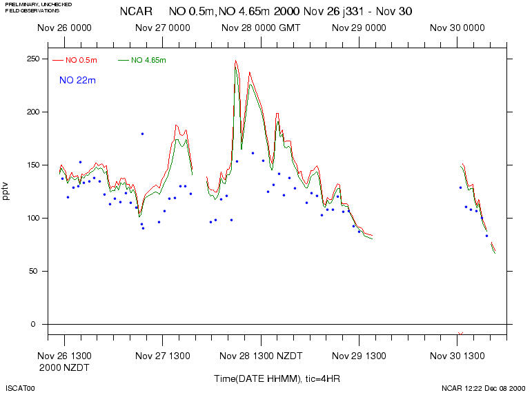
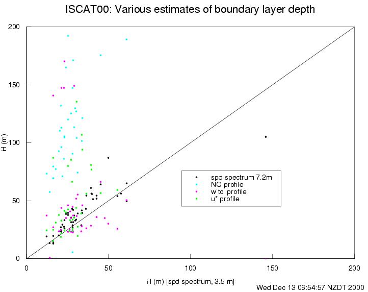
For the same period, I've also plotted the 22m NO concentrations along with the measurements at 0.5 and 4.65m. I've also plotted a typical profile of several quantities. In this case, the height of the boundary layer ("H") has been found by extrapolating the NO concentration or fluxes to a value of 0. The values found, respectively, are 91, 25, and 46m. This is one of the best cases. At Don Lenschow's suggestion, I've also tried to calculate H from the peak in the horizontal wind speed spectra. For this case, it also works out to ~40m. Using all of these methods, I have a plot comparing all H estimates.
Current snow and ice conditions, courtesy of the University of Illinois. (I thought this was interesting!)
[an error occurred while processing this directive]
This page was prepared by
Steven Oncley,
NCAR Research Technology Facility
/html>