NCPLOT User's Guide
Version 4.12.3
Table Of Contents
- Overview
- Getting Started
- Acquiring
- Environment
- Fonts
- Command line options
- Variable Selection Window
- Moving around in Time
- Selecting plot type
- Axes
- Panels
- Selecting and Deselecting variables
- Options
- XY and XYZ additional options
- Plot Canvas
- Canvas features
- Annotations
- Resizing canvas windows
- Zooming
- Menu accelerators
- Guide to menus
- File menu
- Data files
- Templates
- Printing
- Save PNG (GIF substitute)
- Edit Menu
- Editing plot parameters
- View Menu
- ASCII
- Statistics
- Variable Titles
- netCDF header
- Spectra, Cospectra, Quadrature, Phase and Coherence
- Options Menu
- Expression Parser/User Calculations
- Regressions
- Spectral Window
- Features
- Detrending, Segment lengths, and Windowing functions
- Band Limited Variance
- Equal-log interval averaging
- Time shifting (co-spectra)
- Plot Options
- How is my Spectrum being computed?
- Configuration File
- GMT Geo-Political Map Installation
- Known problems
Overview
ncplot is an interactive plotting tool for workstations running X11/R5,
Motif 1.2. ncplot allows the user to view time-series data stored in
netCDF
files that conform to the
NCAR-RAF/nimbus
conventions. Both Low-rate and Mixed-rate files are supported, as well as
files where the data have been reduced below 1 sps (sample per second), e.g.,
files run through ncav.
A few of its features are:
- Plots up to 8 datasets per graph.
- Can draw from up to 4 netCDF files on the same plot.
- 1 to 4 time-series strip charts.
- 1 to 4 XY plots.
- XYZ plot.
- ASCII window.
- Spectra, Co-spectra, Quadrature, Coherence, and Phase.
- Allows user-defined titles, labels, scaling, and major & minor tic marks.
- Annotations.
- Publication quality [Encapsulated] [color] PostScript printouts.
- Optional realtime/on-board mode.
ncplot is NOT for contouring, image or vector data.
ncplot was written at the Research
Aviation Facility of The National
Center for Atmospheric Research to view and analyze our aircraft data
(and NOAA's GIV). The
NCAR-RAF/nimbus
conventions were designed to store multi-rate data, i.e., variable A may be
stored at 5sps and variable B at 25sps. ncplot will plot variables of
differing rates (and from different files) next to each other. Every effort
has been made to make it "what you see is what you get" between the screen
and printouts.
Getting Started
Acquiring
- ncplot is available at https://github.com/ncar/ncplot.
Environment
- ncplot is written in C, requiring X11/R6 and Motif 1.2 (or later),
and the netCDF library 3.0 or later. Specifically it is developed
and maintained on Redhat Enterprise Linux. Builds on most, if not all, Linux
derivatives and MacOS using Homebrew, also availble through MacPorts.
ncplot uses, though it is not required, a shell environment variable
called DATA_DIR as the default directory to locate data files.
The Landmarks button on the track window looks in the directory defined by
the environment variable PROJ_DIR to locate WINDS landmarks
file. If PROJ_DIR points to /home/local/proj, and you are
looking at data from ACE-1, (which is project number 130), then ncplot
will look for the file /home/local/proj/130/landmarks. The project
number is stored in the header of the netCDF file and can be viewed from
the netCDF Header option under the View menu, or with the
netCDF utility program ncdump.
As of 2006 we have started to embed landmarks in the netCDF file as a global
attribute.
Fonts
- Fonts can be over-ridden in the file fbr.h.
Command Line Options
-
-t hh:mm:ss-hh:mm:ss, allows time segment to be entered on command line.
-s template_file, load a template file at startup.
data_file, a netCDF data file that conforms to the
NCAR-RAF/nimbus
conventions.
Examples
- Run with no command line parameters:
1024% ncplot
Load a single data file:
1025% ncplot /home/data/817rf15.cdf
Using everything:
1025% ncplot -s ~/sounding -t 02:00:00-03:00:00 /home/data/181rf15.cdf
Variable Selection Window

Moving around in Time
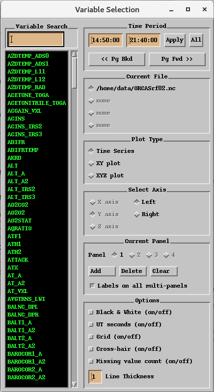
- ncplot comes up with the first 30 minutes of the file as the starting
time frame. New time frames may be entered in the Time Period area
at the top of the Variable Selection window, and then pressing Apply.
PgFwd and PgBkd buttons exist to facilitate moving through the
file in a sequential manner. The Page buttons will keep the same
time frame length until End-of-File is reached; then the time frame may change
to whatever amount of time is remaining in the file. Subsequent PgBkd
will maintain the new time frame length.
The time frame may also be changed in the time-series plots via the
zoom option.
If the flight wraps around midnight, times past midnight should be greater
than 24:00:00 (e.g. 1:00am start time should be entered as 25:00).
Plot Type
- Three primary plot types are supported, time-series, XY, and
XYZ. When you move from one plot type to another, your previous plot
is not lost. To select a plot type, click on its button.
When you select XY or XYZ plot types, a window with additional
options pops up.
Keep in mind that, if you have all the plot types loaded with variables and
move around in time, ALL the variables will be reloaded from all the plots
(including wind vectors), and this may have a serious impact on execution
speed.
Axes
- The various plot types have different active axes. (Inactive axes
are in gray and cannot be selected.)
For the time-series plot, only the Y axis is valid, but you may
select whether future variables you select will be labeled on the right
or left side of the graph.
The XY plot has valid X and Y axes. When the Y axis is selected,
you may choose left or right. The XY plot maps each X with a Y
until one axis runs out of variables, then all remaining variables in
the longer list will be mapped to the last variable in the shorter list.
This allows for doing things like overlaying a GPS track plot on top of
a INS track plot without getting "cross-product" traces drawn.
The XYZ plot only supports one variable on each axis; therefore, there
is no "de-selecting" of variables; just select the new variables you want.
Panels
- Panels are for time-series and XY plots. This
allows you to have up to 4 strip-chart panels in one window for
time-series or 4 vertical profile style panels for XY plots.
Select which panel you want to add or delete variables from. Use the
Add and Delete buttons to add and remove panels. The
Clear button will remove all selected variables from the current panel.
Selecting and Deselecting Variables
- After you have selected which data file, plot type, panel, axis
and location, just click on the variable you wish to select.
- To de-select a variable, click on it again. The file, axis, location and panel must all match from when the variable was selected. This can get confusing if you are drawing data from multiple files. When things get out of hand, you can can clear all variables from the current plot via the Options menu.
The Variable Search allows the user to quickly subset the visible list of variables based on the text typed into this box.
Options
-
- Black & White (on/off)
- Converts all color traces to black and white. Dashed lines are used
to differentiate variables in black and white. This option is provided
to let the user preview monochrome printing.
- UT seconds (on/off)
- Changes time format to seconds since midnight on time-series plots
only.
- Grid (on/off)
- Turns grid on or off for time-series, XY, and XYZ plots.
- Tracking (on/off)
- Provides cross-hair target across all plots, displaying engineering values
of the center of the cross hair.
- Missing value count(on/off)
- Scans time-series data for gaps and displays a count of missing values on the
plot.
- Line thickness
- Let's you select how thick the data traces will be.
XY and XYZ additional options (separate window)
- Much of this window is oriented toward flight track plots. This window
is only effective for XY and XYZ plots.

Flight Tracks
- The INS Track and GPS Track buttons are convienence
functions to quickly load the variables from the respective instruments. In
the case of the XYZ plot, Pressure Altitude is loaded. The variable
names used are currently hard-coded into the software (LAT, LON, [PALT], and
GLAT, GLON, [GALT]). ncplot will load as many of the variables as
it can find (e.g. GALT is routinely not output, and therefore nothing will
be loaded for the Z axis in the XYZ plot when GPS Track is
pressed).
- The Landmarks file is the same one used by WINDS
(see the Environment section for details on location). Below is
the file from ACE-1:
-42.83 147.52 Hobart 1
-43.05 147.08 Huonville 1
-43.64 146.82 SEcape 1
-43.57 146.04 SWcape 1
-42.157 145.80 Strahan 1
The trailing value of zero or one is not used by ncplot, but is
relevant to WINDS.
- The geo-political map makes use of the GMT coastline and
geo-political maps. See appendix on GMT Installation.
- Track scaling is a convenience button to over-ride autoscaling and "square up" the track plot. Degrees lat and lon are converted to a distance based on median lat, and then equal delta X and delta Y are computed.
Wind vectors
- Wind vectors may be added to the XY plot only. (We decided
it would look too confusing on the XYZ plot.) Select whether you
would like averaged or instantaneous vectors, and the
interval in seconds that you would like them displayed. You may
also change the variables you wish to be used. If wind vectors are already
turned on when you change the variables, you must turn them off and then
back on to reload the new variables.
Miscellaneous options
-
- Direction arrows
- Enter the number of direction arrows desired in the text box.
- Time stamps
- Enter the number of time-stamps desired in the text box.
- Scatter plot
- Changes line segments to dots, for XY only.
- Project to XY-plane
- Projects a trace of the XYZ plot onto the XY plane.
- Project to back plane
- Projects a trace of the XYZ plot onto the back and side planes.
Canvas Features
- Annotate
- ncplot has the ability to annotate graphs. In the upper
right corner of the main plot canvas there are a couple of buttons,
one with the letter "A". Press the "A", and your pointer
will turn into a text insertion style cursor. Move the cursor to where
you would like to start the annotation, and press the left mouse button.
Start typing, and finish the annotation by pressing return. Doing
just about anything will clear all annotations (due to the difficulty of
tracking their location as the user moves around in time, and rescales axes).
They should be added as the final option before printing.
- Resize
- All plot canvas windows are fully resizable. In the case of the
spectral window, some buttons will get clipped off the screen.
Resizing the screen will have no affect on sizing or proportion
of your printout, this is controlled via the Printer Setup option.
- Zoom
- A zoom feature exists; place the mouse in the upper left corner
of what you want to zoom in on, hold the left mouse button down, and drag the
box over the segment you want to see. Moving left or above the initial
point will cancel the zoom when you let go. Your mileage may vary if
autoscaling is turned on. There is a un-zoom located in the
Options menu.
- Menu accelerators
- When looking through the various menus, one will notice CTRL
sequences to the right of the menu option label. These are called
menu accelerators, in ncplot they only work while the
cursor is located in the plot canvas.
Guide to Menus
File Menu
- The items in the File menu allow opening of data files from disk,
printer setup, and printing. In the case of an operation that will
overwrite an existing file, you will be prompted by an alert that allows
you to abort the write if you don't want the file to be overwritten.
- Open Data File.
- This displays a File Selection Box to select a file to read. There
is no error checking to see if the input file is valid. Invalid files
tend to cause a segmentation fault. Open Data File will close out all
previously-opened files.
- Add Data File.
- This displays a File Selection Box to select an additional file to open.
- Save Template.
- Save current plot to disk file for future retrieval. Note, file names and
time slices are not saved, this just saves the plot type, number of panels,
the current variables, and User Calculations.
- Load Template.
- Load a previously saved template. This will clear the current plot that
matches the plot type in the template file. You must already have a file
open.
- Save PostScript.
- This displays a File Selection Box prompting for the name of the file
where you want to write the PostScript output.
- Printer Setup.
- This pops up a window with options to change the 'lp' command, the size of
plot to be printed, whether to print landscape or portrait, and color vs.
black and white.
- Print.
- This opens a pipe and sends PostScript commands to lp(1).
- Save PNG.
- This option allows you to save the plot image as a graphics file, which
can then be used in web pages, etc. You can adjust the size of the image
saved by first sizing the plot canvas.
Edit Menu
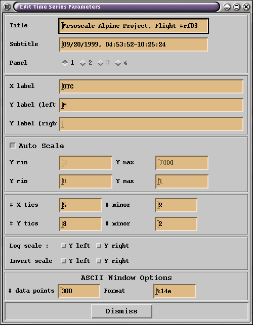
- The Edit Parameter windows allow the user to edit titles, labels,
autoscaling, number of tic marks, log vs. linear, and scale inversion for
each of the plots or windows.

- Time Series Parameters.
- This pops up a window showing all the parameters that are user modifiable
for the main plot window (also contains ASCII options).
- XY Parameters.
- This pops up a window showing all the parameters that are user modifiable
for the XY plot.
- XYZ Parameters.
- This pops up a window showing all the parameters that are user modifiable
for the XYZ plot.
- Spectral Parameters.
- This pops up a window showing all the parameters that are user modifiable
for the spectral window.
- Note: When displaying log scales and auto-scaling is off, the min's and
max's you choose should be powers, not absolute values (i.e. the value you
enter will become 10^x).
View Menu
-
- ASCII.
- This opens a window for viewing the data in ASCII format. Some options
pertaining to this are available in the 'Edit Plot Parameters' menu item.
Note: Because it is possible so many points may be displayed on the graphs
the ASCII window only displays the first 300 (by default) points. Furthermore,
only the first 60 points are printed. However, the save button pops up a
file selection window allowing you to save the entire time segment to a file
of your choice. If the Spectral window is open, then the ASCII window
will display the frequency domain output.
- Variable Titles.
- This opens a window listing variables names and their titles. The
"Category" menu may be used to reduce the list to just variables that belong
in a given category. The category system is not perfect, our system allows a
variable to exist in 1 category, even though some variables should belong in
more than one category.
- netCDF Header.
- This opens a window with output from the ncdump(1) program.
- Statistics.
- This opens a window displaying statistics from all variables currently
being used by ncplot.
- Spectrum.
- This opens a window with Log/Log plot, showing the Power Spectral Density
of the first variable currently being displayed on the main plot window.
- Co-Spectra, Quadrature, Coherence, and Phase.
- This opens a window with Linear/Log plot, showing, whichever of the
above four options, the first two variables currently being displayed
in the main plot window. Sample rates must match.
Options Menu
-
- Un-zoom.
- The drag-zoom has a stack, choose Un-zoom repeatedly to back out.
- Clear current plot.
- Remove all variables from the currently visible plot (Time-series, XY,
or XYZ).
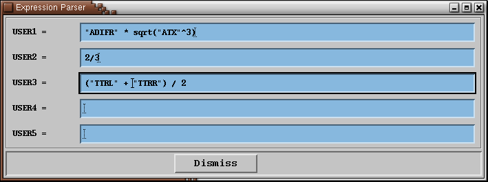
- User Calculations.
- Pops up a window allowing the user to enter their own calculations.
Upto 5 variables can be defined using complex algebraic expressions. Variable
names are case-sensitive and must be quoted. The new variables show up at the
bottom of the variable list in the control window (USER1, USER2, etc). Only
the variables defined will show up.

All of the standard arithmetic operators are available plus the following
intrinsic functions:
sqrt() = Square root.
ln() = Natural log.
log() = log base 10.
exp() = Exponential.
sin() = Sine.
cos() = Cosine.
tan() = Tangent.
abs() = Absolute value.
^ = Power (e.g. 2^3 would be 2 cubed).
- Clear regression.
- Remove all regresions being displayed.
- Linear regression.
- Perform a linear regression, and display the equation's line. Statistics
from the regression are output to the window ncplot was started from.
Regressions currently only available on XY plot.
- Polynomial regression.
- Prompts user for polynomial order (2nd through 5th), then performs the
regression, and displays the curve. Statistics from the regression are
output to the window ncplot was started from. Regressions currently only
available on XY plot.
Spectral Window
Features
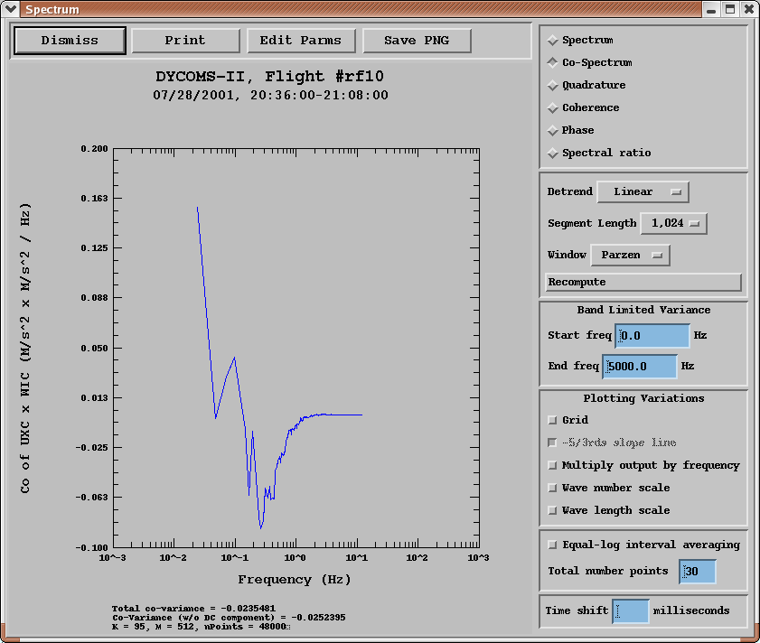
A spectrum is computed from the first variable in the time-series
window, using the same time segment. Co-spectra, quadrature, coherence, and
phase are computed from the first two variables being displayed in the
time-series window.
Along the top row are three buttons, Dismiss and Print should
be obvious. Sizing, lp command, and orientation from the Printer
Setup window will be effective. The Edit Parms button is a
convenient short cut to the Edit menu item of the same name.
The first group of "radio buttons" in the upper right corner are also
short cuts to the items listed under the View menu of the same
name, which allow you to conveniently toggle between the various spectral
displays.
The next group, consists of three "option menus", and a recompute button.
These items control some of the power spectrum density computations.
The first menu is the Segment length to be used by the FFT, and
indirectly determines how many segments will be averaged together. The
second menu is the Windowing function to be applied to each segment.
The third menu determines what type of Detrending to apply to the
entire time-series data. (It is not applied to each segment.) See How
is my spectrum being computed, below, for more details. You must press the
Recompute button to have the changes in any of these menus take affect.
You will notice that two variances are shown at the bottom of the
display. Total variance is always displayed, and the sum includes
the 0th point or DC component of the Pxx spectrum array. The second
variance listed is the Band Limited Variance. By default this
is just the total variance minus the DC component. However you may change
the Start frequency or End frequency to get the variance
computed over a specified interval. The Start/End frequencies will
be truncated down to the nearest bin, no partitioning of these bins will occur.
Time-shifting for co-spectrum is supported. While you
may enter a value to the nearest millisecond, the data will only be
shifted to the nearest sample. For example, if you are doing spectra
on 25sps data, the gap between samples is 40 milliseconds, anything less
than 40 milliseconds that you enter will be truncated to 0, and anything
between 40 and 79 will be truncated to 40 milliseconds or 1 sample.
Equal-log interval averaging may be turned on to reduce the noise
being displayed. You may choose how many points to display, however some
number less than that will actually be displayed due to some bins having
no values to average in.

Plot Options
- Grid - applies a grid to the plot.
- Multiply output by frequency - does just that; only works for
spectrum as it is the default for co-spectrum.
- Wave length scale - may be added to the top of the plot
(TASX required).
- Wave number scale - can replace the bottom frequency scale
(TASX required).
How is my spectrum being computed?
The entire time series data shown in the main ncplot window is
detrended with the user-selected detrend function, and padded
with zeroes on each end, to bring the data length up to a 2 to
the N power. (The FFT algorithm used requires this.) K is incremented
by 2 to make sure every real point is used twice.
The detrended data are then scaled by two different factors, one to
compensate for the effect of zero padding, and the other to compensate
for the effect of windowing.
The Welch peridiogram is then applied. Data segments (of length 2M)
are window'ed, FFT'ed, and summed into Pxx. Each segment overlaps
the previous segment by 50%. Parzen, Welch, and Hanning are among
the best windows to choose from.
Pxx is averaged by dividing by K * Wss * 2M.
Configuration File
ncplot will read a file titled .ncplotrc in your home directory,
if it exists. The following options may be overridden:
Colors = a list of seven colors space and/or comma seperated.
PrintCommand = new print command (eg: lp -d color -o nobanner).
PrintColor = Color (default is B&W).
LineWidth = # (default is 1).
TemplateDirectory = Directory path
TrueAirspeed = TAS variable name (default is TASX).
GpsLongitude = GPS LON variable name (default is GLON).
GpsLatitude = GPS LAT variable name (default is GLAT).
GpsAltitude = GPS ALT variable name (default is GALT).
InertialLongitude = INS LON variable name (default is LON).
InertialLatitude = INS LAT variable name (default is LAT).
PressureAltitude = Pressure ALT variable name (default is PALT).
Colors = red,blue,green,yellow,maroon,orange,
PrintCommand = lp -d color -o nobanner
PrintColor = Color
LineWidth = 2
TemplateDirectory = /home/users/chris/.templates
GpsLongitude = GGLON
GpsLatitude = GGLAT
GpsAltitude = GGALT
The Unix command showrgb(1) can be used to view a list of all available
color names (showrgb | more). The Colors option allows you to override
the plot trace colors.
GMT Geo-Political Map Installation
The geo-political map makes use of the
GMT pscoast sub-command.
For GMT installation from source the GMTHOME environment variable must
be defined for ncplot to engage mapping. The gmt command
must be in your $GMTHOME/bin, and the coast libraries
$GMTHOME/lib/binned_*.cdf (~75Mb) must be installed.
Pre-canned packages exist for Ubuntu/Debian, RHEL/CentOS, MacOSX, and Windows. Usually called 'gmt' or 'GMT'.
For RHEL/CentOS installs, the gmt-gshhg package is missing the high-resolution netCDF files,
so I downloaded those
my self and copied the files into /usr/share/gshhg-gmt-nc4.
Known Problems
- Using the window manager X to close or dismiss a window will cause a core dump. Use 'Dimiss' buttons.
- If the menu and button text shows up as squares, then some fonts are missing.
'yum install "xorg-x11-fonts-ISO8859-1*"' should solve the problem.
- Time gaps in the netCDF file. Time gaps should be filled with _FillValue or
missing_value.
- Invalid data files may cause a core dump.
- No minor tic marks exist for Y axis on XYZ plot.
Author
Christopher J. Webster
National Center for Atmospheric Research
Research Aviation Facility.
email Chris Webster
Last update:
Fri Sep 20 10:16:39 MDT 2024

