Project #1999-102 INDOEX
NSF/NCAR EC-130Q Hercules (N130AR)
Correlation Analysis of LWC Data
The LWC measurements from the FSSP-100s, Hot-wire LWC sensors, and PVM-100 have been analyzed by computing correlation coefficients and doing linear regressions to find the best-fit slopes. The PVM-100 and hot-wire LWC values are those that were in the netCDF files in the productiondata directory on August 15. The FSSP LWC values were computed from the raw counts and used sample volume computed from the product of DOF, Effective beam diameter, and true airspeed at a rate of 1 sample per second (sps). The DOF remained fixed at 2.81 mm, beam diameter = 0.19 mm, and effective beam diameter = 0.6 x beam diameter. No corrections were made for dead-time and coincidence. Flights RF01-RF03 used the left wing pod FSSP and the remaining flights used the right wing pod FSSP. PLWCC and the PVM were on the left wing while PLWCC1 was on the right wing. The cloud data are one-second points defined as those times when the FSSP measured more than 50 cm-3 for at least three seconds (approximately 300 meters in cloud). There are six combinations evaluated: PVM Vs FSSP, PLWCC Vs FSSP, PLWCC1 Vs FSSP, PLWCC Vs PVM, PLWCC1 Vs PVM, PLWCC Vs PLWCC1. The values of the best-fit slope, m, and the Pearson correlation coefficient, r2, have been tabulated in the table below for each combination of instruments and every flight. A r2 > 0.5, indicates statistical significance at the 95% confidence level. As noted in the QC report that I issued last week, the PVM was not available for analysis on flights RF04, RF05 and RF08. PLWCC was also not available on Flight RF04.
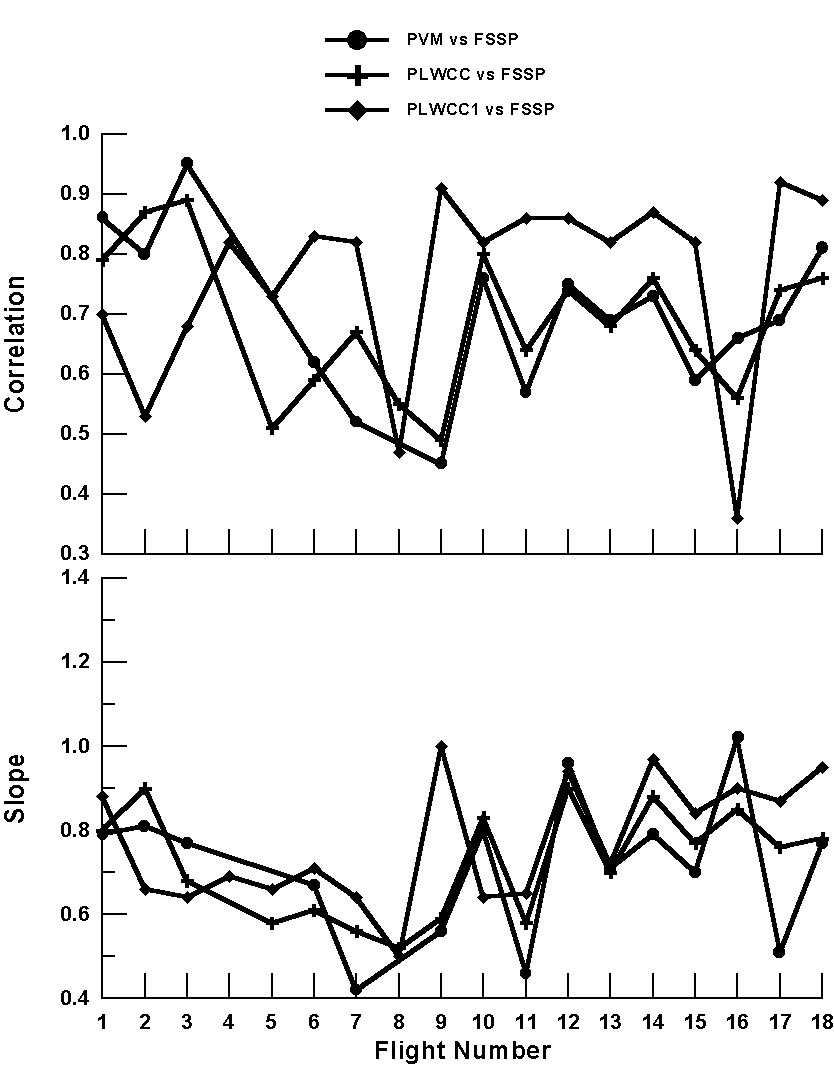
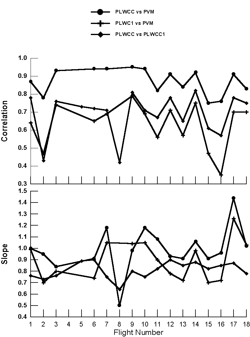
A number of important observations can be made from the data in this table and conclusions drawn. When the data are presented graphically (Figures 1 and 2), these conclusions become even more obvious. First of all, as would be expected, those instruments having the best correlations are those that are located on the same wing. For flights RF01 to RF03, when the left-wing FSSP was used in the analysis, the correlation of the FSSP with PLWCC and the PVM is greater than 0.8 while somewhat less with PLWCC1. For flights RF04 to RF18, the correlation between the right-wing FSSP and PLWCC1 is > 0.8 but < 0.7 with PLWCC and the PVM. Similarly, the correlation between the PVM and PLWCC is almost 0.9 up until flight RF08, then somewhat lower after that. The correlations of PLWCC1 with PLWCC and the PVM are normally < 0.7. This information should be quite interesting from a cloud microphysical point of view, since it provides a rough measure of cloud structure, i.e. that there is still fairly good correlation at distances represented by the separation of the instruments.
The analysis of the best-fit slopes gives us some additional information about instrument performance. Looking at Fig. 1, we see that slopes of the three sensors with respect to to the FSSP gradually decrease, indicating that the FSSP is indicating larger LWCs than the other probes and is doing so more and more over time. This trend is reversed after flight RF07 when the slopes begin to increase with respect to the FSSP for a few flights, and then stabilizes more or less at constant values with respect to the different probes. Since all of the slopes change in more or less the same fashion, this implies that something in the FSSP was changing. There is one possible explanation for the downward trend and two explanations for the upward trend in slopes. The downward trend could have been caused by a gradual increase in the DOF as a result of changing optical alignment. Since I processed with a fixed DOF, a physical increase in DOF would result in larger sample volume and higher perceived concentrations, and hence erroneously larger LWCs. The upward trend could have been caused by a shift in alignment that decreased the DOF with an opposite effect on the measured LWC. An alternative and more plausible explanation is that the optics became contaminated with time, and the instrument gradually undersized particles more and more, with a result that the LWC was underestimated. The measurements made of DOF indicated that there had been a shift from 2.81 when Bill and I measured it soon after his arrival. I believe this was after flight RF07 when we cleaned the optics and aligned the probes at that time. This seems to coincide with the change in trend of the slopes, as well. The post-project measurement indicated a DOF of 1.55. This is a factor of 1.8 shift in the DOF. The slopes change by at most 1.3 if the relationship between PLWC1 and FSSP are used as an indicator of shifts in the FSSP. This would appear to show that either there was something not right about the post-project DOF measurement, or that something occurred on the ferry flights after the final research flight whereby the alignment shifted. In either case, the value of 1.55 should not be used for the DOF. If Cindy's measurement with the CVI support the idea of a slow alignment shift in the FSSP, rather than a decay in optical transmission due to dirty optics, then we can make the decision to adjust the DOF on a flight-by-flight basis and use the FSSP/PLWCC1 ratio to determine the factor.
The other interesting detail shown by the slope analysis is the relationship between PLWCC and PLWCC1. PLWCC is normally about 15% lower than PLWCC1. I don't know if the processing used the correction factor suggested by Krista, but this analysis indicates one of two things: PLWCC or PLWCC1 is being multiplied by a correction factor but shouldn't be, or neither PLWCC or PLWCC1 has the correction factor applied, but one of them should have. Since the SHEBA analysis indicated that the two probes were in near agreement without the correction factor, I suspect that this processing is using a correction factor, but it shouldn't.
I have found this analysis to be very enlightening and plan to implement it as a normal methodology for all future data sets. If it is implemented in the field, it will help us detect shifts in instrument performance. In post-project analysis, it will improve our QC and possibly allow some improvement in processing algorithms.
INDOEX
Least Squares Regression Analysis
m = slope of best fit line
r2 = Pearson Correlation coefficient
|
Flt # |
PVM vs FSSP |
PLWC vs FSSP |
PLWC1 vs FSSP |
PLWC vs PVM |
PLWC1 vs PVM |
PLWC vs PLWC1 |
|
1 |
m = 0.79 R2 = 0.86 |
m = 0.80 R2 = 0.94 |
m = 0.88 R2 = 0.70 |
m = 1.00 R2 = 0.87 |
m = 0.99 R2 = 0.64 |
m = 0.76 R2 = 0.78 |
|
2 |
m = 0.81 R2 = 0.80 |
m = 0.90 R2 = 0.87 |
m = 0.66 R2 = 0.53 |
m = 0.95 R2 = 0.78 |
m = 0.70 R2 = 0.47 |
m = 0.73 R2 = 0.48 |
|
3 |
m = 0.77 R2 = 0.95 |
m = 0.68 R2 = 0.89 |
m = 0.64 R2 = 0.68 |
m = 0.84 R2 = 0.93 |
m = 0.80 R2 = 0.74 |
m = 0.76 R2 = 0.76 |
|
4 |
---------------- |
---------------- |
m = 0.69 R2 = 0.82 |
---------------- |
---------------- |
---------------- |
|
5 |
---------------- |
m = 0.58 R2 = 0.51 |
m = 0.66 R2 = 0.73 |
---------------- |
---------------- |
m = 0.89 R2 = 0.73 |
|
6 |
m = 0.67 R2 = 0.62 |
m = 0.61 R2 = 0.59 |
m = 0.71 R2 = 0.83 |
m = 0.91 R2 = 0.94 |
m = 0.74 R2 = 0.65 |
m = 0.90 R2 = 0.72 |
|
7 |
m = 0.42 R2 = 0.52 |
m = 0.56 R2 = 0.67 |
m = 0.64 R2 = 0.82 |
m = 1.18 R2 = 0.94 |
m =1.05 R2 = 0.69 |
m = 0.75 R2 = 0.71 |
|
8 |
---------------- |
m = 0.52 R2 = 0.55 |
m = 0.50 R2 = 0.47 |
---------------- |
---------------- |
m = 0.64 R2 = 0.42 |
|
9 |
m = 0.56 R2 = 0.45 |
m = 0.59 R2 = 0.49 |
m = 1.00 R2 = 0.91 |
m = 0.98 R2 = 0.95 |
m =1.04 R2 = 0.79 |
m = 0.80 R2 = 0.81 |
|
10 |
m = 0.80 R2 = 0.76 |
m = 0.83 R2 = 0.80 |
m = 0.64 R2 = 0.82 |
m = 1.18 R2 = 0.94 |
m =1.05 R2 = 0.69 |
m = 0.75 R2 = 0.71 |
|
11 |
m = 0.46 R2 = 0.57 |
m = 0.58R2 = 0.64 |
m = 0.65 R2 = 0.86 |
m = 1.08 R2 = 0.82 |
m =0.90 R2 = 0.56 |
m = 0.82 R2 = 0.67 |
|
12 |
m = 0.96 R2 = 0.75 |
m = 0.90 R2 = 0.74 |
m = 0.94 R2 = 0.86 |
m = 0.93 R2 = 0.91 |
m =0.78 R2 = 0.71 |
m = 0.90 R2 = 0.78 |
|
13 |
m = 0.71 R2 = 0.69 |
m = 0.70 R2 = 0.68 |
m = 0.72 R2 = 0.82 |
m = 0.91 R2 = 0.84 |
m = 0.72 R2 = 0.57 |
m = 0.85 R2 = 0.65 |
|
14 |
m = 0.79 R2 = 0.73 |
m = 0.88 R2 = 0.76 |
m = 0.97 R2 = 0.87 |
m = 1.06 R2 = 0.92 |
m = 0.98 R2 = 0.75 |
m = 0.88 R2 = 0.82 |
|
15 |
m = 0.70 R2 = 0.59 |
m = 0.77 R2 = 0.64 |
m = 0.84 R2 = 0.82 |
m = 0.91 R2 = 0.75 |
m = 0.70 R2 = 0.47 |
m = 0.82 R2 = 0.61 |
|
16 |
m = 1.02 R2 = 0.66 |
m = 0.86 R2 = 0.56 |
m = 0.90 R2 = 0.36 |
m = 0.96 R2 = 0.76 |
m = 0.72 R2 = 0.35 |
m = 0.86 R2 = 0.57 |
|
17 |
m = 0.51 R2 = 0.69 |
m = 0.76 R2 = 0.74 |
m = 0.87 R2 = 0.92 |
m = 1.44 R2 = 0.91 |
m = 1.26 R2 = 0.70 |
m = 0.87 R2 = 0.78 |
|
18 |
m = 0.77 R2 = 0.81 |
m = 0.78 R2 = 0.76 |
m = 0.95 R2 = 0.89 |
m = 1.02 R2 = 0.83 |
m = 1.03 R2 = 0.70 |
m = 0.78 R2 = 0.75 |

Figure 1

Figure 2