Every effort was made to preserve every bit and byte of data generated by S-PolKa during DYNAMO. The radar generated approximately 6 TB of original, non-replaceable data, and another 9 TB of differently-formatted data, thresholded/filtered data, or value-added and derived products. Additionally, SMART-R data, some DOE data, and aircraft flight tracks were archived on the S-Pol network (an additional 2 TB).
S-Pol employed two RAID rack-mounted systems with the intention of recording fully redundant data sets. To facilitate return of data from the field, a decision was made to use inexpensive removable disks connected to S-Pol computers via USB interface. Recording of this transfer data set was done in pairs, with the expectation that one or another of the USB disks might fail upon playback.
Ensuring that all data were properly appearing in a complete way on all four disks (two RAIDs and two USB disks) required regular monitoring. A Matlab routine was created that opened all files on all disks, and inventoried the timestamps of the radar beams. Graphical output was generated. The routine was designed to run in batch just after the end of each UTC day.
Additional monitoring was engineered into the Nagios routines, where the fraction of use of the USB disks was updated several times per hour. This real-time monitoring would provide any early tip-off that a disk was in the process of failing.
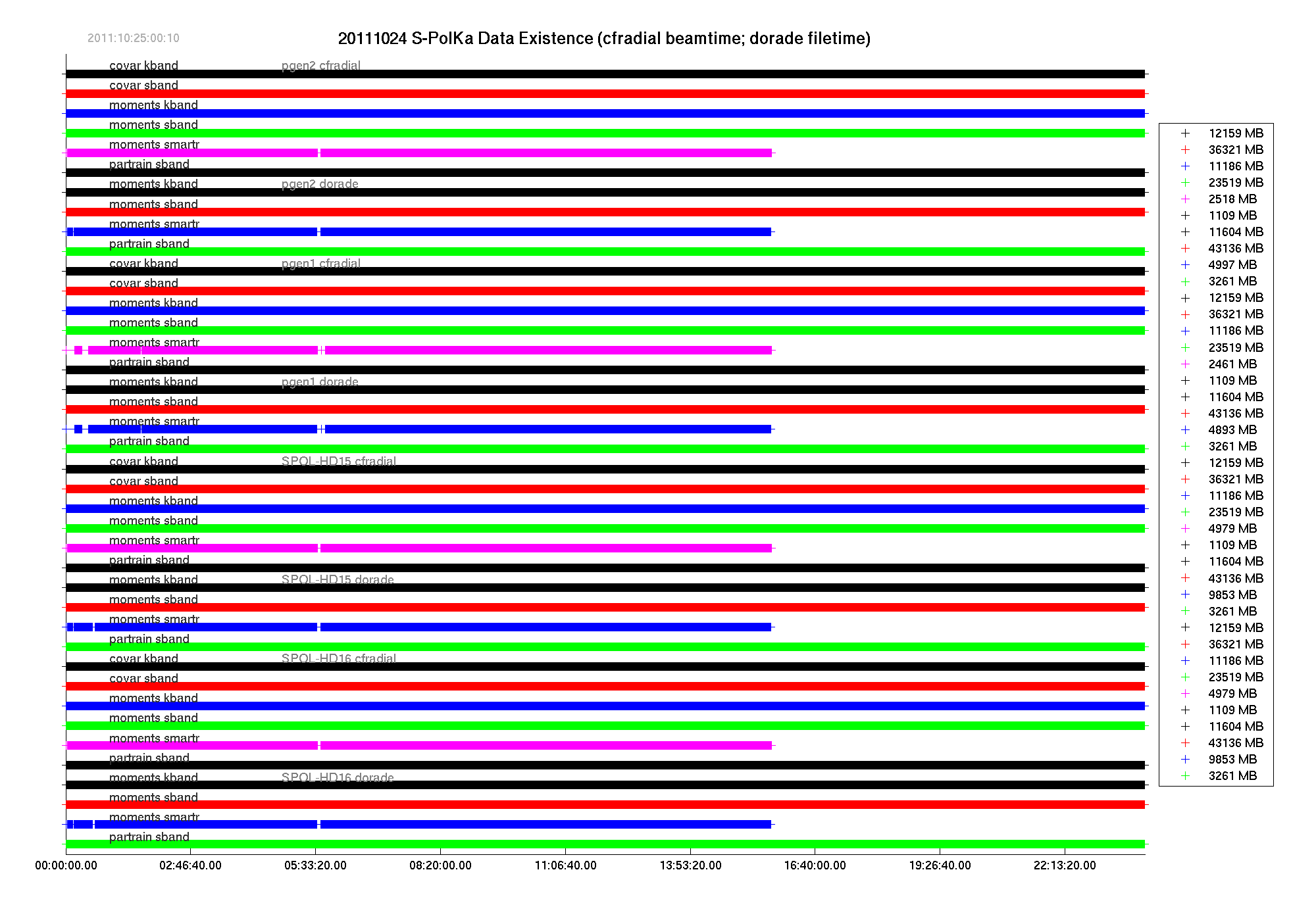
An example of the Matlab time-line graphical summary is shown, below.
The Matlab timeline was responsible for assisting in catching several data recording problems during the shake-out phase of the experiment. Specifically:
The timeline monitoring also contributed to determining when, or if, one of the two different USB disks were failing.
The data time lines were generated using Matlab code. The code ran in batch at the end of each UTC day. Images were saved as png files, but could also be saved as Matlab "fig" files. The "fig" files can be zoomed to any level, allowing analysis of data recording on a beam-by-beam basis.
The main_timeline_multi_plot.m routine is
available here.
Subroutines may be found in this directory.
Note that all removable disks have digital volume labels. Those labels have the format SPOL-HDnn, where "nn" is the two-digit disk number. The main archive RAID systems were named pgen1 and pgen2. The disk names/labels appear in the plot. Since S-PolKa recorded the S-band and K-band data in separate files and directories, there will be separate timelines for each of those sub-systems. SMART-R data were also saved at S-Pol as a backup for the SMART-R. All combinations of radar systems, data formats, and disks are shown in the plot. The total number of MBytes for the day (for each system, format, and disk) are shown on the far right.
Four sets of disks are analyzed, and results should ideally be the same for each disk. Any discrepancies were flagged for further examination and determination of cause for mis-match.
Times on the plot are UTC. Each plot is made up of a series of "+" symbols that tend to run together to form a continuous bar. For CfRadial data files, a "+" is generated for each and every beam of data; for DORADE files, a "+" is plotted for each scan file time (DORADE files were not opened and read, but only inspected for file time stamp and file size).
In-field generated timelines for most days may be found here. (Note: for unknown reasons, in-field timelines were not generated for 11/21 thru 11/30, 12/15 and 01/01.)
Since the USB disks were inexpensive commodity disks, there was a concern that failure rate might be high. All disks were formatted, "pre-burned", and re-formatted as part of a certification effort. Pre-burning consisted of completely filling a disk with patterns of zeros and ones, and monitoring the write speed of the disks during that operation. Of 70 disks purchased, five failed certification and were not used. Three additional disks failed or behaved suspiciously in the field, and were removed from service (upon noticing failure, a replacement copy of the disk was generated).
Disks were formatted and volumes were labeled under Linux using a procedure detailed here.
Simply for completeness, and perhaps for reference during our next project, the in-field Disk Handling Procedure (initial version) is here.
One data system recorded a pair of USB drives. Being somewhat paranoid, and recognizing that a data system failure could cause the loss of both removable drives, a second computer was configured to record data in the same way, to a secondary pair of drives. This secondary pair of drives was re-used multiple times, and only pulled from the secondary recording system if one of the drive pairs on the primary system had failed.
