This document is a standard product of NCAR/ATD/RTF which gives an overview of the measurements taken using the Integrated Surface Flux Facility (ISFF) and conditions during this experiment. If you reached this page from a search engine, click here to see the full report, with frames.
Data Access
ASTER data are stored in two forms:
Location
This experiment was located in rangeland near De Graf, Kansas
(about 15 miles north of El Dorado, and 35 miles northeast of Witchita).
This site had gently rolling terrain, with no major obstacles within several
kilometers. The positions of various sites were:
Sensors
The MICROFRONTS Tower Layout shows the locations
of the ASTER towers used for this program. The south tower group was located
approximately 540m north of the ASTER trailers and the north tower group was
another 300m northeast of the south tower group. The critera for selecting
these locations were:
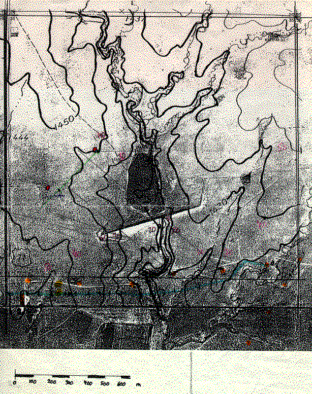
I have prepared a crude map of the section (1 square mile) which has been useful to document the site. This was prepared by photoenlarging the USGS 7.5" topographic map so that it could be overlaid on a photocopy of a blueprint of an aerial photo of the site (taken before the retention dam was built). I've hand embelished this map with red dots for the tower sites, yellow for the trailer locations, and orange for the oil pumps and tanks. (Actually, the towers were at black dots on the thin green line, i.e. the South Towers were about 60m East of the red dot.) A blue line indicates the power line and a high tension line is visible on the lower right. I've put a scale in meters along the bottom, again by hand. The height contour going through the North tower location is 1440 feet and other contours are at 10' intervals.
The MICROFRONTS Configuration documents which sensors were deployed on each of the towers. Each sensor is labeled by the quantities it measures, its name, its height on the tower, and the tower name. Sensor Table lists the type, manufacturer, and other specifications of the sensors used for this project. The south tower group had the majority of sensors, with up to six levels of mean temperature and humidity sensors, three levels of mean wind sensors, two levels of turbulence sensors (three-dimensional sonic anemometer, temperature, and humidity sensors), radiation sensors, a precipitation gauge and soil temperature and heat flux. Both turbulence levels also had mounting locations for hotwire anemometers, though the arrangement of these anemometers changed during the program (see the logbook). The north tower group had fewer sensors, with only two levels mean temperature/humidity sensors, three levels of mean wind sensors, and one sonic anemometer and temperature sensor for turbulence. The setup allowed for a hotwire anemometer to be deployed with this sonic anemometer, but was never used during the program.
The non-standard (not included with ASTER) sensors used for this program were:
Known Instrument Problems
The first half of the program had several periods of heavy rain and/or snow.
Many of the sensors did not perform well in these conditions. Otherwise,
most of the ASTER sensors performed normally. One of the hotwire bridge
circuits died during the early part of the program, so it was never possible
to operate 3 wires.
Albedo from the radiometers should give a good indication of when snow was on the ground (most of the time). Surface conditions (including snow depth) often were noted in the system logbook.
Known instrument problems:
One hotwire was deployed during the last part of setup using one of the Friehe bridges (#1). It ran until an unexpected heavy rain destroyed the (only) probe. Several days later, another probe was deployed. While testing yet another probe with the TSI electronics, that probe died, so we were suspicious of the TSI electronics. The other Friehe bridge (#2) was not working, but recovered after an adjustment was made in its electronics (offset null). At the beginning of the second week of operations, a wire was connected to the Friehe #2 bridge, but it was found that the Friehe #1 bridge had died. Despite extensive work on #1 (replacing all active components), it never recovered. Therefore, data were taken during using #2 for most of the time from week 2 through the end of operations. During the last week of operations, the TSI bridge was tested again and found to work, so about 5 days of data are available with two wires (both on the south towers, and mostly both at 3m in two orientations).
Chronology
Day: Action
The tilt plots show somewhat surprising behavior. The two 10m levels agree quite well, with large (2 degree) angles which generally agree with the slope. However, the 3m.S sonic is nearly flat.
Daily Weather Plots
THE PLOTS IN THIS SECTION ARE NOT FINAL.
The following plots summarize conditions during each day of the project. Each plot covers one Julian day (0000-2359 GMT) and is labeled with time in GMT at the bottom and local time (CST) at the top. The top panel displays temperature and specific humidity from the 3m south tower, pressure, and precipitation rates (if present). Below that is a plot of wind speed and direction from the 10m south tower, with dotted lines showing the directions in which flow distortion by the towers should not be a problem (there may be more). The next panel shows net radiation measured at the south tower, and sensible and latent heat flux from either 3m or 10m on the south tower. (Frequently one of these sensors was bad due to the Krypton hygrometer problems or breakage of the fast temperature probes.) The bottom panel shows the Monin-Obukhov stability parameter, z/L, the friction velocity, u*, and the Bowen ratio calculated from the 3m or 10m south data. Since these fluxes and derived parameters are based on smoothed, 5-minute average statistics, they should not be used quantitatively and are only shown for guidance in selecting periods to analyze further.
Instrument Status Plots
These plots show when there were gaps in the data collected for each
instrument group. These plots do not indicate when sensors were providing
good data, only that a signal was recorded.